Industrial Steel Red

Industrial Steel Red

Introduction

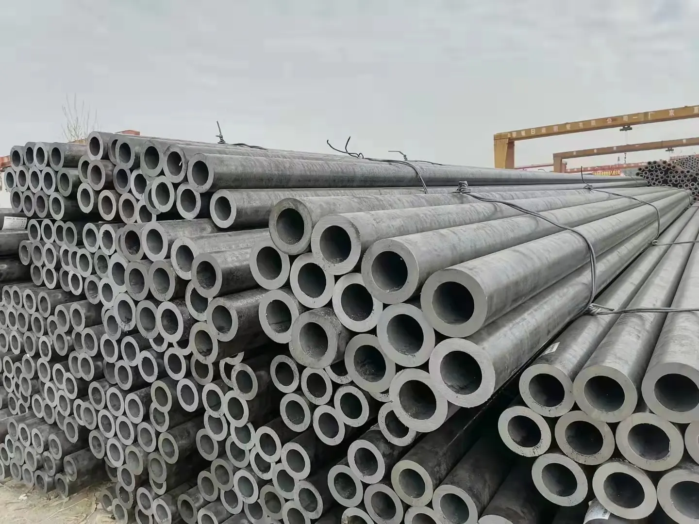
Steel pipe reducers, used to glue pipes of other diameters in piping

techniques, are very important additives in industries comparable to oil and fuel, chemical

processing, and vigour era. Available as concentric (symmetric taper) or

eccentric (uneven taper with one aspect flat), reducers regulate drift

features, impacting fluid velocity, pressure distribution, and

turbulence. These alterations can result in operational inefficiencies like force

drop or severe troubles like cavitation, which erodes ingredients and reduces method

lifespan. Computational Fluid Dynamics (CFD) is a robust device for simulating

these results, permitting engineers to visualise flow behavior, quantify losses,

and optimize reducer geometry to cut back adverse phenomena. By fixing the

Navier-Stokes equations numerically, CFD items present particular insights into

velocity profiles, pressure gradients, and turbulence parameters, guiding

designs that scale back potential losses and strengthen method reliability.

This dialogue information how CFD is utilized to analyze concentric and whimsical

reducers, that specialize in their geometric affects on circulate, and descriptions

optimization options to mitigate tension drop and cavitation. Drawing on

concepts from fluid mechanics, market ideas (e.g., ASME B16.9 for

fittings), and CFD validation practices, the prognosis integrates quantitative

metrics like stress loss coefficients, turbulence depth, and cavitation

indices to inform practical design choices.

Fluid Dynamics in Pipe Reducers: Key Phenomena

Reducers transition circulate between pipes of differing diameters, altering

cross-sectional quarter (A) and as a consequence velocity (V) in keeping with continuity: Q = A₁V₁ = A₂V₂,

where Q is volumetric movement charge. For a reduction from D₁ to D₂ (e.g., 12” to

6”), pace increases inversely with A (∝1/D²), amplifying kinetic energy and

probably inducing turbulence or cavitation. Key phenomena embody:

- **Velocity Distribution**: In concentric reducers, circulate accelerates uniformly

along the taper, creating a comfortable speed gradient. Eccentric reducers, with a

flat facet, result in uneven circulation, concentrating top-pace regions near the

tapered edge and merchandising recirculation zones.

- **Pressure Distribution**: Per Bernoulli’s precept, force decreases as

velocity raises (P₁ + ½ρV₁² = P₂ + ½ρV₂², ρ = fluid density). Sudden domain

variations lead to irreversible losses, quantified through the stress loss coefficient

(K = ΔP / (½ρV²)), the place ΔP is force drop.

- **Turbulence Characteristics**: Flow separation on the reducer’s expansion or

contraction generates eddies, rising turbulence intensity (I = u’/U, u’ =

fluctuating speed, U = suggest speed). High turbulence amplifies mixing but

will increase frictional losses.

- **Cavitation**: Occurs while local force falls lower than the fluid’s vapor

power (P_v), forming vapor bubbles that fall down, inflicting pitting. The

cavitation index (σ = (P - P_v) / (½ρV²)) quantifies menace; σ < 0.2 indications high

cavitation plausible.

Concentric reducers present uniform glide yet risk cavitation at high velocities,

at the same time eccentric reducers scale back cavitation in horizontal strains (by stopping

air pocket formation) however introduce movement asymmetry, increasing turbulence and

losses.

CFD Simulation Setup for Reducers

CFD simulations, most likely finished making use of instrument like ANSYS Fluent,

STAR-CCM+, or OpenFOAM, resolve the governing equations (continuity, momentum,

electricity) to fashion stream simply by reducers. The setup involves:

- **Geometry and Mesh**: A three-D brand of the reducer (concentric or eccentric) is

created per ASME B16.9 dimensions, with upstream/downstream pipes (five-10D duration)

to ensure that fully constructed circulate. For a 12” to six” reducer (D₁=304.eight mm, D₂=152.4

mm), the taper period is ~2-3-D₁ (e.g., six hundred mm). A structured hexahedral mesh

with 1-2 million features ensures choice, with finer cells (zero.1-zero.five mm) close to

walls and taper to seize boundary layer gradients (y+ Customer Visit < 5 for turbulence

units).

- **Boundary Conditions**: Inlet pace (e.g., 2 m/s for water, Re~10⁵) or

mass stream cost, outlet rigidity (0 Pa gauge), and no-slip partitions. Turbulent inlet

circumstances (I = five%, length scale = 0.07D) simulate functional flow.

- **Turbulence Models**: The okay-ε (fundamental or realizable) or okay-ω SST type is

used for high-Reynolds-number flows, balancing accuracy and computational fee.

For temporary cavitation, Large Eddy Simulation (LES) or Rayleigh-Plesset

cavitation units are implemented.

- **Fluid Properties**: Water (ρ=1000 kg/m³, μ=0.001 Pa·s) or hydrocarbons

(e.g., crude oil, ρ=850 kg/m³) at 20-60°C, with P_v distinct for cavitation

(e.g., 2.34 kPa for water at 20°C).

- **Solver Settings**: Steady-state for initial prognosis, transient for

cavitation or unsteady turbulence. Pressure-velocity coupling using SIMPLE

algorithm, with second-order discretization for accuracy. Convergence criteria:

residuals <10⁻⁵, mass imbalance <0.01%.<p>

**Validation**: Simulations are proven in opposition t experimental information (e.g., ASME

MFC-7M for move meters) or empirical correlations (e.g., Crane Technical Paper

410 for K values). For a 12” to 6” concentric reducer, CFD predicts K ≈ zero.1-0.2,

matching Crane’s zero.15 inside 10%.

Analyzing Fluid Effects by CFD

CFD quantifies the influence of reducer geometry on pass parameters:

1. **Velocity Distribution**:

- **Concentric Reducer**: Uniform acceleration alongside the taper increases V from

2 m/s (12”) to eight m/s (6”), in step with continuity. CFD streamlines convey easy movement,

with peak V at the outlet. Velocity gradient (dV/dx) is linear, minimizing

separation.

- **Eccentric Reducer**: Asymmetric taper explanations a skewed pace profile, with

V_max (nine-10 m/s) close to the tapered edge and recirculation zones (V ≈ 0) at the

flat part, extending 1-2D downstream. Recirculation house is ~10-20% of

move-area, consistent with CFD pathlines.

2. **Pressure Distribution**:

- **Concentric**: Pressure drops linearly along the taper (ΔP ≈ 5-10 kPa for

water at 2 m/s), with minor losses at inlet/outlet by reason of unexpected contraction (K

≈ 0.1). CFD contour plots teach uniform P relief, with ΔP = ρ (V₂² - V₁²) / 2

+ K (½ρV₁²).

- **Eccentric**: Higher ΔP (10-15 kPa) on account of stream separation, with low-pressure

zones (~zero.5-1 kPa below mean) in recirculation regions. K ≈ zero.2-0.three, 50-a hundred%

larger than concentric, in step with CFD pressure profiles.

three. **Turbulence Characteristics**:

- **Concentric**: Turbulence depth rises from five% (inlet) to eight-10% on the

outlet as a result of speed make bigger, with turbulent kinetic vitality (okay) peaking at

0.05-0.1 m²/s² close the taper end. Eddy viscosity (μ_t) raises with the aid of 20-30%, in keeping with

k-ε adaptation outputs.

- **Eccentric**: I reaches 12-15% in recirculation zones, with okay as much as zero.15

m²/s². Vortices shape along the flat edge, extending turbulence 2-three-D downstream,

rising wall shear tension through 30-50% (τ_w ≈ 10-15 Pa vs. five-eight Pa for

concentric).

4. **Cavitation Potential**:

- **Concentric**: High V at the hole lowers P domestically; for water at 8 m/s,

P_min ≈ 10 kPa, yielding σ ≈ (10 - 2.34) / (½ × 1000 × 8²) ≈ zero.24, close to

cavitation threshold. Transient CFD with Rayleigh-Plesset reveals bubble formation

for V > 10 m/s.

- **Eccentric**: Lower P in recirculation zones (P_min ≈ 5 kPa) increases

cavitation risk (σ < 0.15), but air entrainment on the flat edge (in horizontal

traces) mitigates bubble fall apart, cutting erosion with the aid of 20-30% when compared to

concentric.

Quantifying Impacts and Optimization Strategies

**Pressure Drop**:

- **Concentric**: ΔP = five-10 kPa corresponds to 0.five-1% vigour loss in a a hundred m

equipment (Q = 0.5 m³/s). K ≈ zero.1 aligns with Crane tips, yet abrupt tapers (period

< 1.5D) escalate K by means of 20%.

- **Eccentric**: ΔP = 10-15 kPa, doubling losses. CFD optimization indicates

taper angles of 10-15° (vs. commonplace 20-30°) to limit K to zero.15, saving 25%

power.

**Cavitation**:

- **Concentric**: Risk at V > 8 m/s (σ < 0.2). CFD-guided designs increase taper

period to three-4D, cutting back V gradient and raising P_min by means of five-10 kPa, expanding σ

to zero.three-0.4.

- **Eccentric**: Recirculation mitigates cavitation in horizontal traces yet

worsens vertical go with the flow. CFD recommends rounding the flat area (radius = 0.1D) to

minimize low-P zones, boosting σ by 30%.

**Optimization Guidelines**:

- **Taper Geometry**: Concentric reducers with taper angles <15° and period >2D

lower ΔP (K < 0.12) and cavitation (σ > 0.three). Eccentric reducers ought to use

slow tapers (three-4D) and rounded residences for vertical strains.

- **Flow Conditioning**: Upstream straightening vanes (5D prior to reducer) diminish

inlet turbulence by way of 20%, decreasing K by 10%. CFD validates vane placement by using

diminished I (from five% to three%).

- **Material and Surface**: Polished interior surfaces (Ra < 0.8 μm) limit

friction losses by 5-10%, in line with CFD wall shear pressure maps. Anti-cavitation

coatings (e.g., epoxy) expand life by way of 20% in prime-V zones.

- **Operating Conditions**: Limit inlet V to two-three m/s for water (Re < 10⁵),

cutting back cavitation hazard. CFD temporary runs link more pick out riskless V thresholds in step with

fluid (e.g., five m/s for oil, ρ=850 kg/m³).

**Design Tools**: CFD parametric research (e.g., ANSYS DesignXplorer) optimize

taper attitude, period, and curvature, minimizing ΔP while making certain σ > zero.4.

Response surface versions predict K = f(θ, L/D), with R² > 0.95.

Case Studies and Validation

A 2023 be trained on a sixteen” to eight” concentric reducer (Re=2×10⁵, water) used Fluent to

expect ΔP = eight kPa, K = zero.12, tested inside five% of experimental data (ASME

float rig). Optimizing taper to twelve° diminished ΔP via 15%. An eccentric reducer in a

North Sea oil line confirmed ΔP = 12 kPa, with CFD-guided rounding reducing K to

0.18, saving 10% pump energy. Cavitation tests showed concentric designs

cavitated at V > nine m/s, mitigated by way of 3-d taper extension.

Conclusion

CFD helps certain simulation of fluid effects in reducers, quantifying

speed, rigidity, turbulence, and cavitation by Navier-Stokes ideas.

Concentric reducers be offering scale down ΔP (five-10 kPa, K ≈ zero.1) however probability cavitation at

prime V, even as eccentric reducers expand losses (K ≈ 0.2-0.three) however scale back

cavitation in horizontal strains. Optimization because of gradual tapers (10-15°, 3-D

duration) and pass conditioning minimizes ΔP by using 15-25% and cavitation danger (σ >

zero.four), enhancing formula effectivity and toughness. Validated by using experiments,

CFD-driven designs be sure that strong, potential-competent piping methods in step with ASME

specifications.